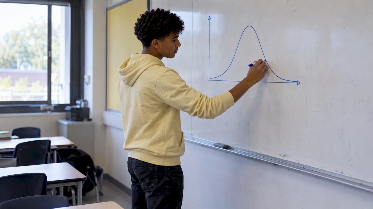
The normal distribution is a continuous, bell-shaped model that is symmetrical about its mean. At A-Level you use it in three ways: finding probabilities with a calculator, working backwards from a probability to a value, and (on some specifications) approximating a binomial distribution. Almost every exam question reduces to one habit: define the variable, standardise if you need to, draw a sketch, then use your calculator.
This guide takes you through each skill in order, with worked examples you can try before reading the solution, the mistakes examiners see most often, and where to find real exam questions to practise on.
TL;DR
- Write X ~ N(μ, σ²). The second number is the variance, so the standard deviation is its square root. Mixing these up is the most common lost mark.
- Sketch a bell curve and shade the region every time. It catches wrong-way-round answers before they cost you marks.
- To find a probability, use your calculator’s normal cumulative function. To find a value from a probability, use the inverse normal function.
- If a question gives you two probabilities and asks for μ and σ, standardise both and solve simultaneous equations.
- To approximate a binomial, match the mean and variance, then apply a continuity correction of ±0.5. Check your exam board’s specification first, because boards differ.
Table of Contents
- What the normal distribution is, and what μ and σ do
- What your specification requires
- Finding probabilities: the standard method
- Working backwards: inverse normal questions
- Normal approximation to the binomial
- Common mistakes and how to avoid them
- How to practise so the method sticks
- Practise with real exam questions
- What we think about learning this topic
- Get the full set of practice papers
- FAQ
- Sources
What the normal distribution is, and what μ and σ do
The normal distribution, also called the Gaussian distribution, is shown as a bell-shaped curve. Its peak sits at the mean, and the standard deviation measures how spread out the probabilities are. In exam notation, X ~ N(μ, σ²) means X follows a normal distribution with mean μ and variance σ².
The two parameters have separate jobs:
- μ (the mean) decides where the peak sits. Change it and the whole curve slides left or right.
- σ (the standard deviation) decides the shape. A large standard deviation gives a short, wide curve, and a small one gives a tall, narrow curve.
The total area under the curve is 1, and area represents probability. Because the variable is continuous, P(X = a) is zero for any single value, so P(X < a) and P(X ≤ a) are identical. That is different from the binomial distribution, and it matters when you reach continuity corrections.
The curve is symmetrical, so P(X < μ − a) = P(X > μ + a). The specifications also expect you to know that the points of inflection are at μ ± σ. OCR’s A-Level Mathematics A specification states this explicitly, and AQA links the Normal model to histograms, mean, standard deviation and points of inflection.
The 68, 95 and 99.7 rule
Roughly 68% of values lie within one standard deviation of the mean, 95% within two and 99.7% within three. Specifications phrase this as about two-thirds within μ ± σ, about 95% within μ ± 2σ and almost all within μ ± 3σ.
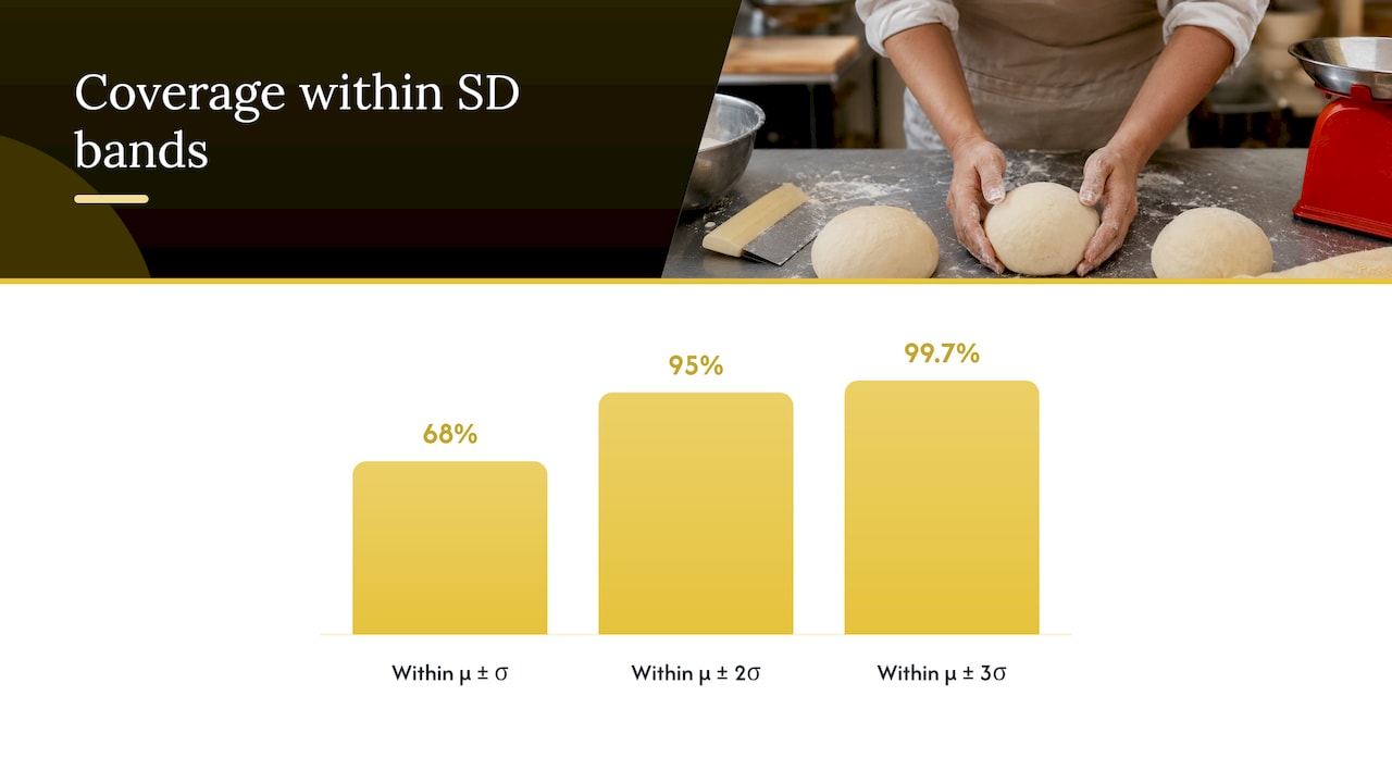
These benchmarks are your sanity check. If you calculate P(μ − σ < X < μ + σ) and get 0.32, you know something has gone wrong, because it should be close to 0.68.
What your specification requires
The content is similar across boards, but the detail is not identical, so read the relevant pages of your own specification.
- AQA (7357): content N2 requires you to understand and use the Normal distribution as a model and find probabilities using it, linking it to histograms, mean, standard deviation, points of inflection and the binomial distribution.
- OCR (H240): the specification requires understanding and using the standard normal distribution Z and standardising, along with the two-thirds, 95% and almost-all benchmarks above. The equation of the normal curve is excluded.
- Older Edexcel S1 (pre-2017): knowledge of the probability density function was not required, and questions could involve solving simultaneous equations. That second point still shows up in modern questions, as the third worked example below shows.
In short, you never need to integrate the normal density by hand. You need to model, standardise, use technology accurately and interpret the answer in context.
Finding probabilities: the standard method
Follow the same five steps every time.
- Define the variable. Write “Let X be the height of a student” and state X ~ N(170, 8²).
- Sketch. Draw the bell, mark μ, and shade the region you want.
- Calculate. Use the normal cumulative distribution function on your calculator, entering lower bound, upper bound, mean and standard deviation.
- Check against the sketch. Is the shaded area small or large? Does your answer agree?
- Answer in context. Write a sentence, not just a decimal.
Worked example 1: a simple upper-tail probability
The heights of Year 12 students are modelled by X ~ N(170, 8²), in cm. Find the probability that a randomly chosen student is taller than 180 cm.
Standardise: z = (180 − 170) ÷ 8 = 1.25.
P(X > 180) = P(Z > 1.25) = 1 − 0.8944 = 0.1056.
So about 10.6% of students are taller than 180 cm. Your sketch shows a small shaded tail, which agrees. Note that 180 is a little over one standard deviation above the mean, and the one-sigma rule suggests the upper tail beyond that should be roughly 16%, so a value a bit smaller than that is sensible.
Why standardisation still matters
Your calculator can often skip the standardising step, but the method is examinable and it is essential for the harder questions below. The transformation is:
Z = (X − μ) ÷ σ
Z follows the standard normal distribution, N(0, 1). A z-value tells you how many standard deviations a value sits from the mean. It lets you compare values from different distributions and turn an unknown μ or σ into an equation.
Between two values
For P(a < X < b), use the calculator with both bounds. Written by hand, it is P(Z < z_b) − P(Z < z_a). If the question asks for the probability of being outside an interval, subtract the inside probability from 1, or double one tail if the interval is symmetrical about the mean.
Working backwards: inverse normal questions
Here you are given a probability and asked for a value. The inverse normal function on your calculator returns the value of x with a given area to its left.
Careful with tails. Calculators give the area to the left. If a question asks for the value exceeded by the top 10%, you need the value with 0.9 to its left.
Worked example 2: the top 10%
Using X ~ N(170, 8²), find the height exceeded by only 10% of students.
We need k such that P(X > k) = 0.1, so P(X < k) = 0.9.
For the standard normal, the z-value with 0.9 to its left is 1.2816 (to 4 d.p.).
k = 170 + 1.2816 × 8 = 180.25, so k ≈ 180.3 cm.
Check: 180.3 is about 1.28 standard deviations above the mean. That sits between the one-sigma and two-sigma benchmarks, which is where a 10% upper tail should be.
Worked example 3: finding μ and σ
The time, T minutes, that a revision video is watched is normally distributed. 20% of viewers watch for less than 40 minutes and 10% watch for more than 60 minutes. Find μ and σ.
From the inverse normal: P(T < 40) = 0.2 gives z = −0.8416, and P(T > 60) = 0.1 gives z = +1.2816.
Write two equations:
- (40 − μ) ÷ σ = −0.8416, so 40 = μ − 0.8416σ
- (60 − μ) ÷ σ = 1.2816, so 60 = μ + 1.2816σ
Subtract the first from the second: 20 = 2.1232σ, so σ ≈ 9.42.
Substitute back: μ = 40 + 0.8416 × 9.42 ≈ 47.9.
The signs are where marks are lost. The lower value is below the mean, so its z-value must be negative. Check: 47.9 lies between 40 and 60, as it must.
Using a single known probability
Sometimes you know σ and one probability, and need μ (or the reverse). The structure is the same: find the z-value, write one equation, solve. Always write the equation in the form (x − μ) ÷ σ = z so that you can show the method even if your arithmetic slips.
Normal approximation to the binomial
A binomial distribution counts successes in a fixed number of trials. When the number of trials is large, its bar chart looks like a bell, so a normal distribution can approximate it.
The specification wording differs by board. AQA content N3 requires you to select an appropriate distribution for a context, with reasoning, including recognising when a binomial or Normal model may not be appropriate. Look at the statistics section of your own specification to see whether a worked approximation with a continuity correction is expected, or whether you are only asked to comment on suitability.
When the approximation is reasonable
For X ~ B(n, p), the usual guidance is to check that both np and n(1 − p) are large, often taken as at least 5. The approximation is better when p is close to 0.5, because the binomial is then nearly symmetrical. If p is very small or very large the binomial is skewed, and the normal curve fits poorly.
If you are asked to justify using the approximation, state the condition and then show it holds with numbers, for example np = 30 and n(1 − p) = 70.
The recipe
- Write X ~ B(n, p).
- Find the mean np and variance np(1 − p).
- State the approximation: Y ~ N(np, np(1 − p)).
- Apply the continuity correction.
- Calculate and give your answer in context.
Remember that the second parameter of N is a variance, so you do not square np(1 − p) again. On the calculator, you will need its square root as the standard deviation.
The continuity correction
The binomial takes whole-number values, whereas the normal is continuous. To bridge the gap, each integer r is treated as occupying the interval from r − 0.5 to r + 0.5. The correction is adding or subtracting 0.5 from the discrete value. Use this table:
| Binomial probability | Normal probability to calculate |
|---|---|
| P(X = r) | P(r − 0.5 < Y < r + 0.5) |
| P(X ≤ r) | P(Y < r + 0.5) |
| P(X < r) | P(Y < r − 0.5) |
| P(X ≥ r) | P(Y > r − 0.5) |
| P(X > r) | P(Y > r + 0.5) |
The tricky ones are the strict inequalities. P(X < 35) means X goes up to 34, and 34 covers up to 34.5, so the boundary is 34.5, not 35.5. Write the list of included integers if you are unsure.
Worked example 4
X ~ B(100, 0.3). Use a normal approximation to estimate P(X ≤ 35).
Mean = 100 × 0.3 = 30. Variance = 100 × 0.3 × 0.7 = 21, so σ = √21 ≈ 4.583.
Conditions: np = 30 and n(1 − p) = 70, both comfortably above 5.
Y ~ N(30, 21). With the correction, P(X ≤ 35) ≈ P(Y < 35.5).
z = (35.5 − 30) ÷ 4.583 ≈ 1.20, and P(Z < 1.20) ≈ 0.885.
There is a probability of about 0.885 that at most 35 successes occur. Without the correction you would use 35 and get z ≈ 1.09, a noticeably different answer, which is why examiners award a specific mark for it.
Common mistakes and how to avoid them
These are the slips that most often cost marks on normal distribution questions. They tend to be the same each year.
- Using σ² as σ. If X ~ N(50, 16), the standard deviation is 4, not 16. Underline the variance when you read the question.
- Forgetting that the calculator gives the left tail. For “greater than”, subtract from 1 or use the upper-bound setting.
- Wrong sign of z. Any value below the mean has a negative z. Check against your sketch.
- Rounding z too early. Keep at least four decimal places through the working, and round only at the end, unless the question tells you otherwise.
- Missing the continuity correction, or applying it in the wrong direction. Use the table above.
- No context. Many marks are for interpretation. “0.106” earns less than “the probability that a student is taller than 180 cm is 0.106”.
- Treating a sample as the whole population. Read carefully whether the question concerns a single observation or a mean of several.
- Not justifying the model. If the question asks you to comment on the suitability of a normal model, refer to the context: is the variable continuous, symmetrical, and bell-shaped, and does it cluster around a central value? Real examples include heights, errors in measurements, blood pressure and test marks.
How to practise so the method sticks
Reading worked solutions is a good start, but marks come from doing the questions. A reliable routine for this topic:
- Learn the benchmarks. Be able to state 68%, 95% and 99.7% without hesitation.
- Do five basic probability questions with a sketch each time.
- Do three inverse questions, including one “top x%” and one “middle x%”.
- Do two unknown μ and σ questions, because the algebra needs repetition.
- Attempt the binomial approximation if your board examines it, and write the condition check each time.
- Mark your own work against a mark scheme, noting where method marks and accuracy marks were available.
Official material helps with step 6. AQA’s All About Maths hub has specimen assessment materials, practice papers and teaching guidance for each topic.
Practise with real exam questions
At MathVault we organise A-Level papers by exam board and year, so you can jump straight to the statistics questions and check your working against full mark schemes. If you sit AQA, start with our AQA A-Level Maths past papers and work through the Statistics section of each paper. Our A-Level past-paper questions page is useful when you want to practise by topic rather than by whole paper.
When you are stuck, the way you use a solution matters. Our guide to using A-Level maths walkthroughs to gain marks explains how to try a question first and then use the worked solution to find the exact line where your method diverged. If you prefer to ask a question and get an answer in real time, see how to get the most from A-Level maths live Q&A.
What we think about learning this topic
Normal distribution is a topic where students often feel they understand the idea but still lose marks on the details. That is a feature of the topic, not a weakness in the student. The ideas are few, but the notation, the tail direction and the continuity correction each have a trap in them.
We built MathVault around the belief that the quickest way to close that gap is repeated exposure to real exam questions with fully worked solutions. When you see how a mark scheme awards method and accuracy marks, you start writing answers the way examiners want to read them: a defined variable, a clear standardisation, a stated condition, a sentence in context.
That is why we keep past papers, step-by-step solutions, video walkthroughs and live Q&A together and free to use. A written solution is good for checking a line of algebra, while a video is good when you need to see why a step was chosen. Using both, after you have first attempted the question yourself, is how we think students build lasting confidence.
Oloru
Get the full set of practice papers
Everything you need to revise statistics is free to use on MathVault: past papers, mark schemes, worked solutions, video walkthroughs and a weekly live Q&A. If you want offline access, organised revision packs for your exam board and year range are also available, and small donations help us keep the free resources growing.

Browse maths past papers for AQA, Edexcel, OCR, WJEC and CIE to find your board, or start from our homepage to see every resource in one place.
FAQ
Do I need to memorise the normal distribution table for A-Level?
No. A-Level courses expect you to use your calculator’s normal cumulative and inverse normal functions. You should still understand standardisation and know the 68%, 95% and 99.7% benchmarks, because they help you check that a calculator answer is sensible.
What is the difference between σ and σ² in X ~ N(μ, σ²)?
σ is the standard deviation and σ² is the variance. A normal distribution is written with the variance, so X ~ N(100, 25) has a standard deviation of 5. Enter 5, not 25, in your calculator.
How do I know whether to use a continuity correction?
Use one whenever you approximate a discrete distribution, such as the binomial, with the continuous normal. You do not use one when the original variable is already continuous, such as height or time. Check your specification to see whether your board examines the binomial approximation.
Why is P(X = a) zero for a normal distribution?
For a continuous variable, probability is area under the curve, and a single point has no width, so its area is zero. This is why P(X < a) and P(X ≤ a) are equal for a normal variable.
What should I draw in a normal distribution question?
Draw a symmetrical bell curve, mark the mean on the horizontal axis, label the boundary values, and shade the required region. A quick sketch helps you choose the correct tail and often earns a method mark.
Sources
- Maths in a minute: The normal distribution, Plus Maths
- Measures of average and spread, House of Commons Library
- Statistics review 2: Samples and populations, PubMed Central
- OCR A Level Mathematics A (H240) specification
- AQA A-level Mathematics (7357) specification
- AQA Level 3 Mathematical Studies specification
- Edexcel S1 syllabus (pre-2017)
- AQA All About Maths: A-level Maths
- Continuity correction, Wikipedia
- Normal approximation to binomial, Richland College
Leave a Reply