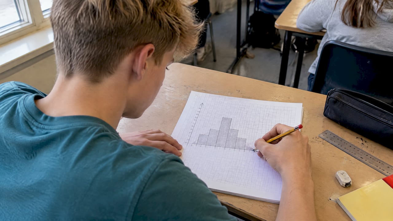
A GCSE histogram is a chart of grouped, continuous data in which the area of each bar, not its height, shows the frequency. When the class widths are unequal, the vertical axis is frequency density (frequency ÷ class width). Almost every histogram mark on the paper comes from knowing when to use that one idea and how to run it in both directions.
This guide takes you through reading, drawing and calculating with histograms, with worked examples, the missing-frequency questions that catch people out, and the mistakes examiners see again and again.
TL;DR
- Bar area = frequency. Height is frequency density, and width is class width.
- Frequency density = frequency ÷ class width. Frequency = frequency density × class width.
- Unequal class widths must give unequal bar widths, with no gaps between bars.
- For missing values, find the area of the known bars first, then use proportion or the total.
- Add a frequency density column to every table before you draw or read anything.
Table of Contents
- What a histogram shows, and why it is not a bar chart
- The three formulas you need
- How to draw a histogram from a grouped table
- How to read a histogram that has already been drawn
- Missing frequencies, widths and heights
- Mistakes that cost marks
- How to practise so it sticks
- Our perspective
- Practise histograms on real exam questions
- FAQ
- Sources
What a histogram shows, and why it is not a bar chart
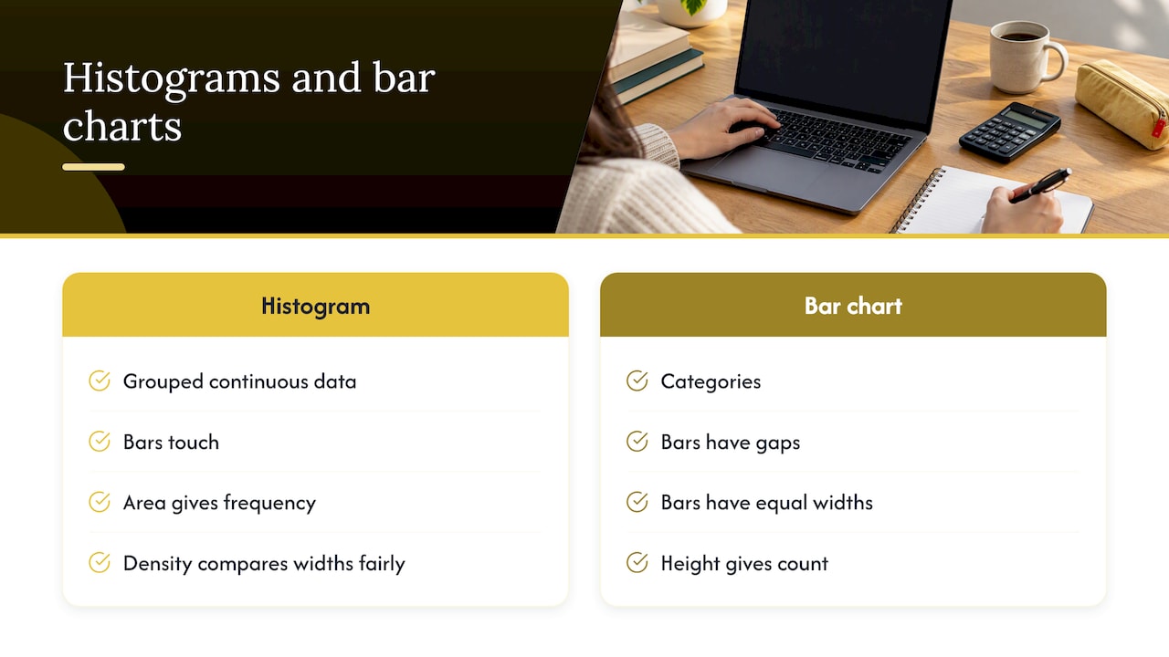
A histogram represents grouped data, and the area of each bar represents the frequency. A bar chart compares categories, so its bars have gaps and equal widths, and height gives the count. A histogram covers a continuous scale such as time, height or mass, so the bars touch.
That is why height alone can mislead. If one class is twice as wide as its neighbour, it will usually contain more people or items for the same height. Frequency density corrects for this. The Open University defines it as frequency per unit of data in a class, which is what lets you compare classes of different widths fairly.
Statisticians use histograms for the same reason you do in an exam: to see the shape of a distribution. The NIST statistical handbook notes that a histogram can reveal centre, spread, skewness, outliers and multiple modes. In a GCSE question, that usually becomes “which class has the most data?” or “describe the distribution”.
Which tier and which boards
Histograms are a Higher-tier topic. BBC Bitesize labels frequency density histograms as Higher only in its WJEC guide. If you sit Foundation, you will meet bar charts, frequency polygons and histograms with equal widths in other contexts, but not the frequency density work. Check your own board’s specification to be sure. To see how often the topic is likely to appear, our GCSE maths topic frequency analysis shows how topics are spread across the papers.
The three formulas you need
Everything in this topic comes from one relationship, written three ways:
| You want | Formula | Notes |
|---|---|---|
| Class width | upper bound − lower bound | Use the boundaries of the class, not the midpoint |
| Frequency density | frequency ÷ class width | This is the bar height |
| Frequency | frequency density × class width | This is the bar area |
BBC Bitesize gives the same method: class width is the upper bound minus the lower bound, and frequency density is frequency divided by that width. You recover frequency by multiplying the other way.
A useful habit: write “FD × width = frequency” at the top of your working before you touch the question. It stops you reading a height as a frequency.
How to draw a histogram from a grouped table
Take this table of the times, in minutes, that 135 students spent on homework one evening.
| Time, t (minutes) | Frequency |
|---|---|
| 0 < t ≤ 10 | 20 |
| 10 < t ≤ 30 | 60 |
| 30 < t ≤ 40 | 25 |
| 40 < t ≤ 60 | 30 |
Step 1: add two columns
Add class width and frequency density. This follows the method BBC Bitesize describes: add the two columns, then calculate each width and density.
| Time, t (minutes) | Frequency | Class width | Frequency density |
|---|---|---|---|
| 0 < t ≤ 10 | 20 | 10 | 2 |
| 10 < t ≤ 30 | 60 | 20 | 3 |
| 30 < t ≤ 40 | 25 | 10 | 2.5 |
| 40 < t ≤ 60 | 30 | 20 | 1.5 |
Step 2: choose your axes
The horizontal axis is a continuous number line for time, from 0 to 60. The vertical axis is frequency density, from 0 to at least 3. Choose a scale that uses most of the grid, with equal steps. Label the vertical axis “Frequency density”, because a bare “Frequency” label can lose a mark.
Step 3: draw the bars
Each bar’s width runs from its lower to its upper boundary, and its height is the frequency density. So you draw a bar from 0 to 10 at height 2, from 10 to 30 at height 3, from 30 to 40 at height 2.5 and from 40 to 60 at height 1.5. The bars touch and do not leave gaps.
Before you move on, check one bar’s area. The 10 to 30 bar has width 20 and height 3, so its area is 60, which matches the frequency. If it does not, find the slip now.
How to read a histogram that has already been drawn
Exam questions often give you the histogram and no table. Start by building the table yourself.
- Read each bar’s boundaries from the horizontal axis and work out its width.
- Read each bar’s height from the vertical axis. Check the scale carefully, as grid squares are often not worth 1.
- Multiply width by height to get the frequency for each class.
- Write the frequencies in a table and total them if you need the whole group.
The OpenLearn text states the rule directly: in a frequency density histogram, frequency equals bar area, class width × frequency density.
Estimating part of a class
Sometimes a question asks how many values lie between 15 and 20 minutes, which falls inside the 10 to 30 class. Assume the data are spread evenly across the class. The width you want is 5 and the bar height is 3, so the estimate is 5 × 3 = 15. The word “estimate” matters here, because you are assuming even spread within the class.
Estimating a median from a histogram
Using the homework example, the total is 135, so the median is the 67.5th value. The first class holds 20 values, and the first two together hold 80. So the median is in the 10 to 30 class, and you need 47.5 more values after the 10-minute mark. At 3 values per minute, that is 47.5 ÷ 3 ≈ 15.8 minutes. The estimated median is about 25.8 minutes.
Missing frequencies, widths and heights
These questions look harder than they are. They give you part of the picture and a piece of information that links the rest. In every case, you are using area = frequency.
Type 1: a bar is missing from the histogram
A table says a class has frequency 18, and its width is 6. The bar height is 18 ÷ 6 = 3. Draw it at that height over its interval.
Type 2: a frequency is missing from the table
You are told the bar over 30 to 35 has height 2.4. The width is 5, so the frequency is 2.4 × 5 = 12. Fill the table, then continue with the question.
Type 3: use a known bar to scale the others
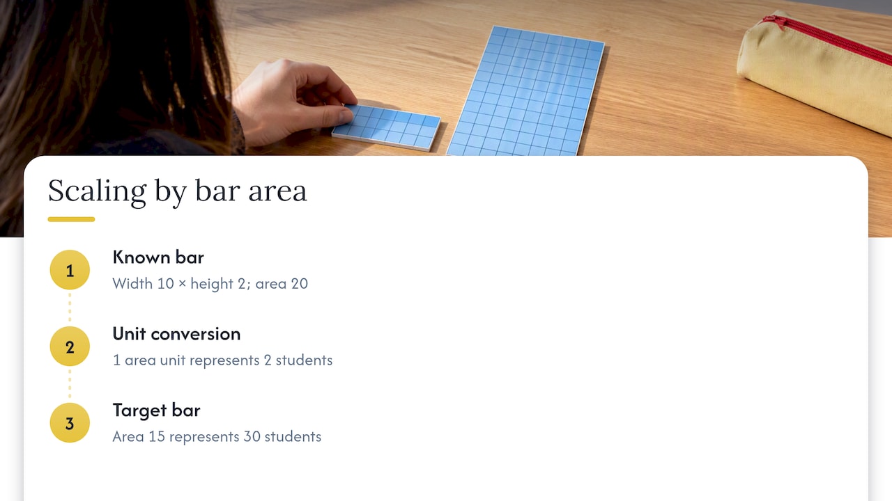
A question may say that 40 students are represented by a bar of width 10 and height 2 on a histogram. Hold on to the scale: that bar has area 20, yet it represents 40. So one unit of area represents 2 students, and a bar with area 15 represents 30. This catches students who simply read heights as frequencies, because the histogram in the question might not have frequency density on the vertical axis at all. If the axis is unlabelled, compare areas.
Type 4: use a total to find an unknown
If the question gives the total frequency, add the known class frequencies, subtract from the total and divide the remainder by the unknown class width to find the missing height. Write each step down, because method marks are available even if your final number is wrong.
Type 5: compare two histograms
When the question asks you to compare distributions, use the area (frequency) for the numbers, then comment on shape and spread, in context. A sentence such as “Class B has a greater proportion of students over 40 minutes” earns more than “Class B is higher”.
Mistakes that cost marks
These are the errors we see most often when students attempt histogram questions. Each has a quick fix.
| Mistake | Why it loses marks | The fix |
|---|---|---|
| Plotting frequency as the height when widths are unequal | The areas no longer represent frequency | Always calculate frequency density first |
| Reading the height as the frequency | You miss the multiplication by width | Write FD × width = frequency before you read anything |
| Drawing bars with gaps | The data are continuous | Make adjoining bars touch |
| Equal-width bars for unequal classes | The class boundaries are misrepresented | Measure each bar from its own boundaries |
| Misreading the vertical scale | The numbers feed every later step | Work out what one small square is worth first |
| Calculating width from the wrong numbers, such as using the midpoint | Every density is then wrong | Take the upper bound minus the lower bound |
| Forgetting to label the axes | Easy marks lost | Write “Frequency density” and the variable with its units |
| Giving an exact answer to an “estimate” question | The even-spread assumption is not stated | Use the word “estimate” in your working |
A quick self-check before you move on
- Does each bar’s width match its class interval?
- Does width × height give a frequency that makes sense for the question?
- Do the frequencies sum to the stated total?
- Have you labelled both axes?
If all four pass, you can be confident about the bars.
How to practise so it sticks
Histogram questions come in only a few shapes, so deliberate repetition works well. Aim for short sessions rather than a single long one.
- Do one drawing question from a table, then one reading question from a drawn histogram. Switching direction is the skill.
- Do the missing-value types listed above until you can name the type in a few seconds.
- Mark your own working against the mark scheme, looking at where the method marks sit. A correct frequency density column alone often earns a mark.
- Mix histograms in with other statistics topics such as cumulative frequency and box plots, because exams do.
If calculators are restricted in your paper, the arithmetic here is friendly, since class widths are usually round numbers. Our guide to non-calculator paper strategy shows how to keep method marks when you do the arithmetic by hand.
Our perspective
Histograms are one of the topics where understanding beats memorising. Students who learn the single idea that area is frequency can handle drawing, reading, estimating and missing-value questions without separate rules for each.
We built our resources around that principle. Our fully worked solutions show every line of method, because that is where the marks are, and our topic-based revision guides separate the concept from the exam technique. We want a student to see not only the answer to a histogram question, but why each step was taken.
Our approach is to keep this support free: past paper questions organised by exam board, step-by-step solutions, video walkthroughs and live weekly Q&A sessions. A question you cannot crack at 9pm on a Sunday should not depend on what your family can pay for help.
Oloru
Practise histograms on real exam questions
Reading about frequency density is the first half. The second half is doing exam-style questions and checking your working against a full solution. We organise past paper questions and revision material by exam board, so you can practise the topic as your own board sets it.
Start with our GCSE maths revision guides for topic notes, then move on to the OCR GCSE maths revision topics or Edexcel past paper questions by topic. If your exam is close, our last-minute GCSE maths revision plan shows how to divide your final days. Taking your studies further, our A-Level maths past-paper questions continue the statistics you meet here.
FAQ
Are histograms on the Foundation or Higher GCSE maths paper?
Histograms with frequency density are Higher-tier content. BBC Bitesize marks the topic as Higher only. Foundation students still work with other grouped-data charts, so check your board’s specification for exactly what is covered.
What is the difference between a histogram and a bar chart?
A bar chart shows separate categories, with gaps between bars of equal width. A histogram shows continuous grouped data, with touching bars. When class widths differ, the histogram’s vertical axis is frequency density and the area of each bar gives the frequency.
How do I find the frequency from a histogram?
Multiply the bar’s width by its height. The height is the frequency density, so this gives the frequency for that class. Do it for every bar if you need a total, and check that your answer is sensible for the context.
Why do I need frequency density at all?
When classes have different widths, a wider class would look larger simply because it covers more values. Dividing frequency by class width gives a fair comparison per unit. This is what OpenLearn recommends for comparing unequal classes.
What should I do if a histogram question gives no table?
Build one. List each class boundary, work out each width and height, and multiply them to get frequencies. A table keeps your working visible, which protects method marks if you slip on a later step.
Sources
- What is a histogram? BBC Bitesize
- Frequency density, Histograms, Higher only, WJEC GCSE: BBC Bitesize
- Data analysis: visualisations in Excel, 2.4 Frequency density: The Open University, OpenLearn
- 1.3.3.14. Histogram: NIST Engineering Statistics Handbook
Leave a Reply